karlen provides real-time PCR data sets by Karlen et al. (2007) in tidy format.
Installation
install.packages("karlen")Data
The raw PCR amplification curve data by Karlen et al. (2007) is provided as one single eponymously named data set: karlen. In the original publication each data set pertaining one PCR plate is provided as a separate spreadsheet file. The column plate in karlen distinguishes each data set.
The karlen data set comprises quantitative real-time PCRs for four samples (S1 thru S4), for seven amplicons targeting seven genes: Cav1, Ctfg, Eln, Fn1, Rpl27, Hspg2, Serpine1.
For each sample/target combination a dilution series was performed. One PCR plate was used per amplicon, except for Rpl27 (L27) that was assayed twice (plates L27_1 and L27_2). The target column indicates the mouse gene symbol matching the targeted amplicon.
library(ggplot2)
library(dplyr, warn.conflicts = FALSE)
library(karlen)

karlen |>
  dplyr::distinct(plate, target, sample, sample_type) |>
  print(n = Inf)
#> # A tibble: 36 × 4
#>    plate target   sample sample_type
#>    <fct> <fct>    <fct>  <fct>
#>  1 CAV   Cav1     S1     std
#>  2 CAV   Cav1     S2     std
#>  3 CAV   Cav1     S3     std
#>  4 CAV   Cav1     S4     std
#>  5 CAV   Cav1     <NA>   ntc
#>  6 CTGF  Ctgf     S1     std
#>  7 CTGF  Ctgf     S2     std
#>  8 CTGF  Ctgf     S3     std
#>  9 CTGF  Ctgf     S4     std
#> 10 ELN   Eln      S1     std
#> 11 ELN   Eln      S2     std
#> 12 ELN   Eln      S3     std
#> 13 ELN   Eln      S4     std
#> 14 ELN   Eln      <NA>   ntc
#> 15 L27_1 Rpl27    S1     std
#> 16 L27_1 Rpl27    S2     std
#> 17 L27_1 Rpl27    S3     std
#> 18 L27_1 Rpl27    S4     std
#> 19 L27_2 Rpl27    S1     std
#> 20 L27_2 Rpl27    S2     std
#> 21 L27_2 Rpl27    S3     std
#> 22 L27_2 Rpl27    S4     std
#> 23 FN    Fn1      S1     std
#> 24 FN    Fn1      S2     std
#> 25 FN    Fn1      S3     std
#> 26 FN    Fn1      S4     std
#> 27 Perl  Hspg2    S1     std
#> 28 Perl  Hspg2    S2     std
#> 29 Perl  Hspg2    S3     std
#> 30 Perl  Hspg2    S4     std
#> 31 Perl  Hspg2    <NA>   ntc
#> 32 PAI1  Serpine1 S1     std
#> 33 PAI1  Serpine1 S2     std
#> 34 PAI1  Serpine1 S3     std
#> 35 PAI1  Serpine1 S4     std
#> 36 PAI1  Serpine1 <NA>   ntc
Two dilution series schemes were assayed:
- Scheme 1 (Cav1, Eln, Hspg2, Serpine1): 1-fold, 10-fold, 50-fold, and 100-fold;
- Scheme 2 (Ctgf, Rpl27, Fn1): 1-fold, 10-fold, 50-fold, 100-fold and 1000-fold (two replicates only).
karlen |>
  dplyr::filter(sample_type == "std") |>
  dplyr::distinct(plate, target, dilution) |>
  print(n = Inf)
#> # A tibble: 36 × 3
#>    plate target   dilution
#>    <fct> <fct>       <int>
#>  1 CAV   Cav1            1
#>  2 CAV   Cav1           10
#>  3 CAV   Cav1           50
#>  4 CAV   Cav1          100
#>  5 CTGF  Ctgf            1
#>  6 CTGF  Ctgf           10
#>  7 CTGF  Ctgf           50
#>  8 CTGF  Ctgf          100
#>  9 CTGF  Ctgf         1000
#> 10 ELN   Eln             1
#> 11 ELN   Eln            10
#> 12 ELN   Eln            50
#> 13 ELN   Eln           100
#> 14 L27_1 Rpl27           1
#> 15 L27_1 Rpl27          10
#> 16 L27_1 Rpl27          50
#> 17 L27_1 Rpl27         100
#> 18 L27_1 Rpl27        1000
#> 19 L27_2 Rpl27           1
#> 20 L27_2 Rpl27          10
#> 21 L27_2 Rpl27          50
#> 22 L27_2 Rpl27         100
#> 23 L27_2 Rpl27        1000
#> 24 FN    Fn1             1
#> 25 FN    Fn1            10
#> 26 FN    Fn1            50
#> 27 FN    Fn1           100
#> 28 FN    Fn1          1000
#> 29 Perl  Hspg2           1
#> 30 Perl  Hspg2          10
#> 31 Perl  Hspg2          50
#> 32 Perl  Hspg2         100
#> 33 PAI1  Serpine1        1
#> 34 PAI1  Serpine1       10
#> 35 PAI1  Serpine1       50
#> 36 PAI1  Serpine1      100
Visualization of amplification curves (NTC curves are omitted):
karlen |>
  dplyr::filter(sample_type != "ntc") |>
  ggplot(aes(x = cycle, y = fluor, group = well, col = as.factor(dilution))) +
  geom_line(linewidth = 0.1) +
  geom_point(size = 0.05) +
  facet_grid(rows = vars(plate), cols = vars(sample), scales = "free_y") +
  labs(color = "Fold dilution")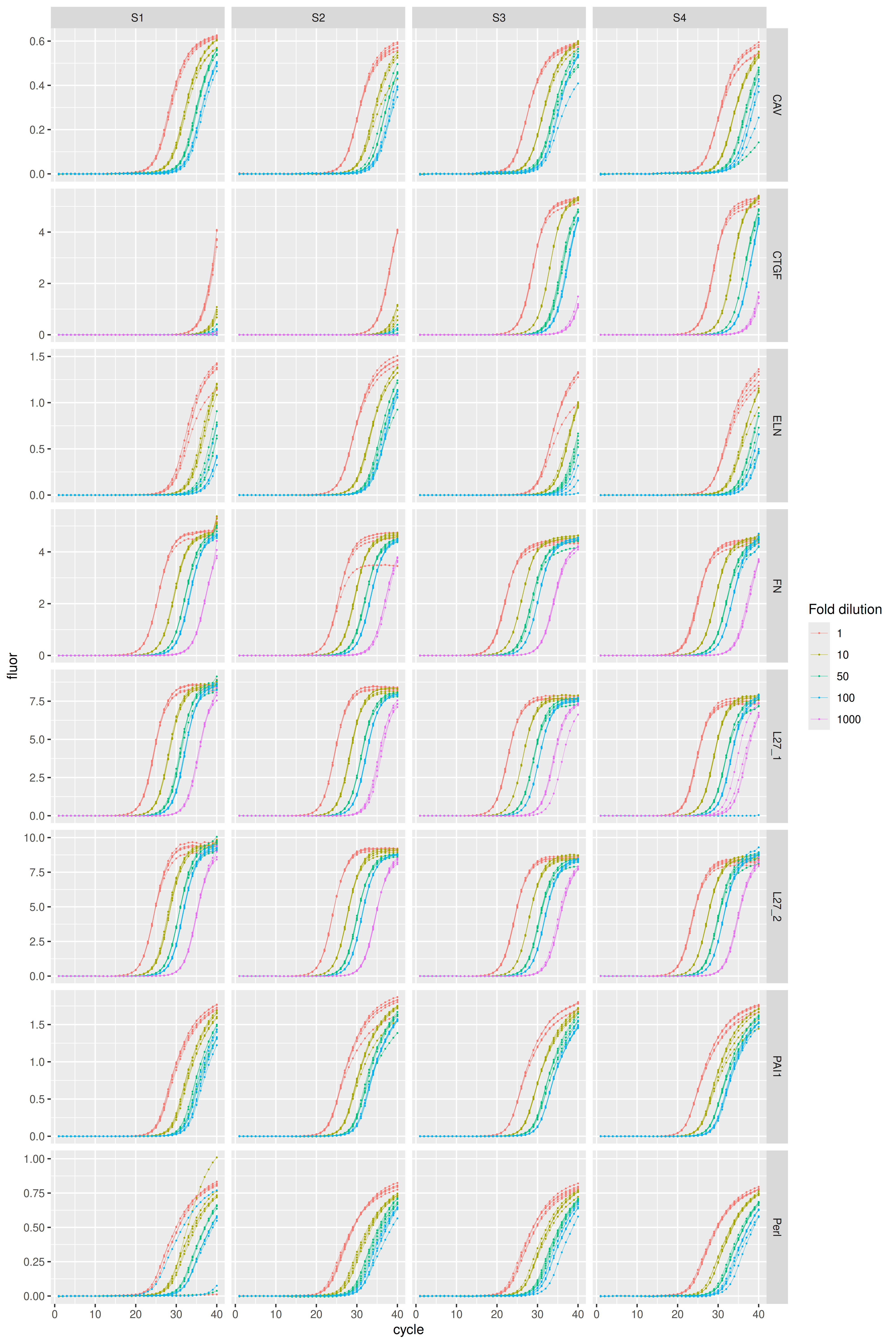
References
Yann Karlen, Alan McNair, Sébastien Perseguers, Christian Mazza, and Nicolas Mermod. Statistical significance of quantitative PCR. BMC Bioinformatics 8, 131 (2007). doi: 10.1186/1471-2105-8-131.